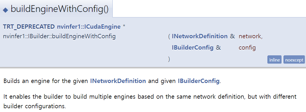
위의 공식 문서에서 제공해주는 Custom pooling layer의 예시를 기준으로 작성하겠습니다.
class PoolPlugin : public IPluginV2IOExt
{
    ...override virtual methods inherited from IPluginV2IOExt.
};
poolPlugin에서는
supportsFormatCombination
configurePlugin
enqueue
위의 세가지 method를 수정해주어야 합니다.
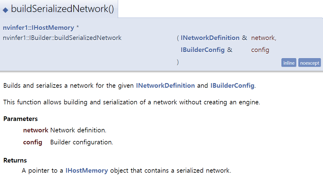
1. network에 Custom layer 추가하기
// Look up the plugin in the registry
IPluginV2 creator = getPluginRegistry()->getPluginCreator(pluginName, pluginVersion);
const PluginFieldCollection* pluginFC = creator->getFieldNames();

//populate the fields parameters for the plugin layer
PluginFieldCollection *pluginData = parseAndFillFields(pluginFC, layerFields);

//create the plugin object using the layerName and the plugin meta data
IPluginV2 *pluginObj = creator->createPlugin(layerName, pluginData);

//add the plugin to the TensorRT network
IPluginV2Layer* layer = network.addPluginV2(&inputs[0], int(inputs.size()), pluginObj);
ITensor* data = layer.getOutput(0);
pluginObj->destroy() // Destroy the plugin object
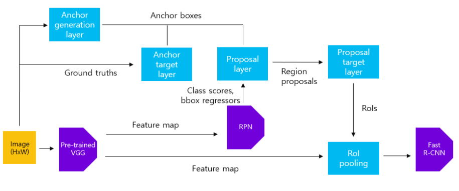
1) 먼저 Anchor generation layer에서 생성된 anchor box와 원본 이미지의 ground truth box를 사용하여 Anchor target layer에서 RPN을 학습시킬 positive/negative 데이터셋을 구성합니다. 이를 활용하여RPN을 학습시킵니다. 이 과정에서 pre-trained된 VGG16 역시 학습됩니다.
2) Anchor generation layer에서 생성한 anchor box와 학습된 RPN에 원본 이미지를 입력하여 얻은 feature maps를 사용하여 proposals layer에서 region proposals를 추출합니다. 이를 Proposal target layer에 전달하여 Fast R-CNN 모델을 학습시킬 positive/negative 데이터셋을 구성합니다. 이를 활용하여Fast R-CNN을 학습시킵니다. 이 때 pre-trained된 VGG16 역시 학습됩니다.
3) 앞서 학습시킨 RPN과 Fast R-CNN에서RPN에 해당하는 부분만 학습(fine tune)시킵니다. 세부적인 학습 과정은 1)과 같습니다. 이 과정에서 두 네트워크끼리 공유하는 convolutional layer, 즉pre-trained된 VGG16은 고정(freeze)합니다.
4) 학습시킨 RPN(3)번 과정)을 활용하여 추출한 region proposals를 활용하여Fast R-CNN을 학습(fine tune)시킵니다. 이 때RPN과 pre-trained된 VGG16은고정(freeze)합니다.
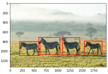
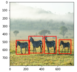
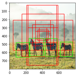
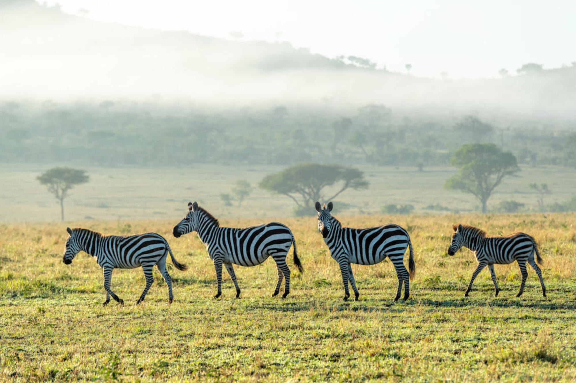
# Resize BBox
w_ratio = 800/origin_img.shape[1]
h_ratio = 800/origin_img.shape[0]

print('w_ratio : {}'.format(w_ratio))
print('h_ratio : {}\n'.format(h_ratio))

ratio_list = [w_ratio, h_ratio, w_ratio, h_ratio]
bbox = []

for box in origin_bbox:
  box = [int(a*b) for a,b in zip(box, ratio_list)]
  bbox.append(box)

bbox = np.array(bbox)
print(bbox)

copy_img = np.copy(img)
for i in range(len(bbox)):
  cv.rectangle(copy_img, (bbox[i][0], bbox[i][1]), (bbox[i][2], bbox[i][3]), color=(255, 0, 0), thickness=5)
plt.imshow(copy_img)
plt.show()
Create Extractor Model
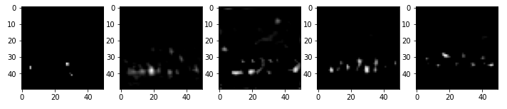
2) VGG16을 통해 feature map을 추출해줍니다.
# Feature extractor

model = torchvision.models.vgg16(pretrained=True).to(device)
features = list(model.features)
print(len(features))
for i, layer in enumerate(features):
  print('{}th Layer : {}'.format(i, layer))
# Visualize output_feature
imgs = output_feature.data.cpu().numpy().squeeze(0)
fig = plt.figure(figsize=(12, 4)) # figsize=전체사이즈
no = 1

for i in range(5):
  fig.add_subplot(1, 5, no)
  plt.imshow(imgs[i], cmap='gray')
  no += 1

plt.show()
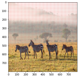
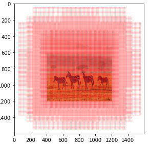
Generate Anchors Boxes
3) Anchor generation layer에서는 anchor box를 생성하는 역할을 합니다. 이미지의 크기가 800x800이며, sub-sampling ratio=1/16이므로, 총 22500(=50x50)개의 anchor box를 생성해야 합니다. 서로 다른 scale과 aspect ratio를 가지는 9개의 anchor box를 생성해줍니다.anchor_boxes변수에 전체 anchor box의 좌표(x1, y1, x2, y2)를 저장합니다(anchor_boxes 변수의 크기는 (22500, 4)입니다).
# Create Anchors Boxes Center
ctr = np.zeros((2500, 2)) # (x, y)

index = 0
for i in range(len(ctr_x)):
  for j in range(len(ctr_y)):
    ctr[index, 0] = ctr_x[i] - 8
    ctr[index, 1] = ctr_y[j] - 8
    index += 1

print(ctr.shape)
print(ctr[:10, :])

# Create Anchors Boxes
ratios = [0.5, 1, 2]
scales = [8, 16, 32]
sub_sample = 16

anchor_boxes = np.zeros(((feature_size * feature_size * 9), 4))
index = 0

for c in ctr:
  ctr_y, ctr_x = c
  for i in range(len(ratios)):
    for j in range(len(scales)):

      h = sub_sample * scales[j] * np.sqrt(ratios[i])
      w = sub_sample * scales[j] * np.sqrt(1./ratios[i])

      anchor_boxes[index, 0] = ctr_x - w/2.
      anchor_boxes[index, 1] = ctr_y - h/2.
      anchor_boxes[index, 2] = ctr_x + w/2.
      anchor_boxes[index, 3] = ctr_y + h/2.
      index += 1

print(anchor_boxes.shape)
print(anchor_boxes[:10, :])
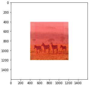
5) RPN을 학습시키기 위한 Positive, Negative Anchor Box를 나눠줍니다.
# Anchor Boxes의 ious 중 가장 큰 값을 가지는 iou 뽑기

# 각 Truth Box 별 가장 높은 iou값의 위치
gt_argmax_ious = ious.argmax(axis=0)
print(gt_argmax_ious)

# 각 Truth Box 별 가장 높은 iou값
gt_max_ious = ious[gt_argmax_ious, np.arange(ious.shape[1])]
print(gt_max_ious)

# 가장 높은 iou값들 추출
gt_argmax_ious = np.where(ious == gt_max_ious)[0]
print(gt_argmax_ious)
# 이미지 내에 있는 8940개의 Anchor Box가 각각 어떤 Truth Box와 연관이 많이 되어있는지
argmax_ious = ious.argmax(axis=1)
max_ious = ious[np.arange(len(index_inside)), argmax_ious]

# Label 정해주기
label = np.empty(len(index_inside), dtype = np.int32)
label.fill(-1)

pos_iou_threshold = 0.7
neg_iou_threshold = 0.3

label[gt_argmax_ious] = 1
label[max_ious >= pos_iou_threshold] = 1
label[max_ious < neg_iou_threshold] = 0
# First set the label=-1 and locations=0 of the 22500 anchor boxes,
# and then fill in the locations and labels of the 8940 valid anchor boxes
# NOTICE: For each training epoch, we randomly select 128 positive + 128 negative
# from 8940 valid anchor boxes, and the others are marked with -1

anchor_labels = np.empty((len(anchor_boxes),), dtype=label.dtype)
anchor_labels.fill(-1)
anchor_labels[index_inside] = label

anchor_locations = np.empty((len(anchor_boxes),) + anchor_boxes.shape[1:], dtype=anchor_locs.dtype)
anchor_locations.fill(0)
anchor_locations[index_inside, :] = anchor_locs
RPN
6) RPN을 정의해 줍니다.
# Send the features of the input image to the Region Proposal Network (RPN),
# predict 22500 region proposals (ROIs)

in_channels = 512
mid_channels = 512
n_anchor = 9

conv1 = nn.Conv2d(in_channels, mid_channels, 3, 1, 1).to(device)
conv1.weight.data.normal_(0, 0.01)
conv1.bias.data.zero_()

# bounding box regressor
reg_layer = nn.Conv2d(mid_channels, n_anchor * 4, 1, 1, 0).to(device)
reg_layer.weight.data.normal_(0, 0.01)
reg_layer.bias.data.zero_()

# classifier (object or not)
cls_layer = nn.Conv2d(mid_channels, n_anchor * 2, 1, 1, 0).to(device)
cls_layer.weight.data.normal_(0, 0.01)
cls_layer.bias.data.zero_()
# For classification we use cross-entropy loss
rpn_cls_loss = F.cross_entropy(rpn_score, gt_rpn_score.long().to(device), ignore_index = -1)
# For Loc Loss
# only positive samples
pos = gt_rpn_score > 0
mask = pos.unsqueeze(1).expand_as(rpn_loc)
# take those bounding boxes whick have positive labels
mask_loc_preds = rpn_loc[mask].view(-1, 4)
mask_loc_targets = gt_rpn_loc[mask].view(-1, 4)
x = torch.abs(mask_loc_targets.cpu() - mask_loc_preds.cpu())
rpn_loc_loss = ((x < 1).float() * 0.5 * x ** 2) + ((x >= 1).float() * (x - 0.5))
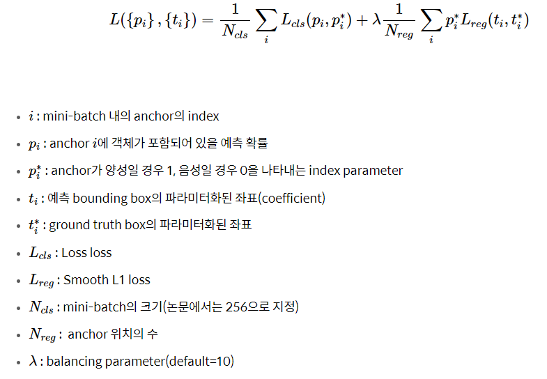
# Combining both the rpn_cls_loss and rpn_reg_loss
rpn_lambda = 10
N_reg = (gt_rpn_score > 0).float().sum()
rpn_loc_loss = rpn_loc_loss.sum() / N_reg
rpn_loss = rpn_cls_loss + (rpn_lambda * rpn_loc_loss)
Proposal Layer
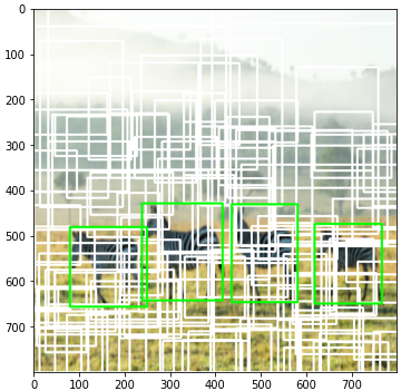
8) Proposal Layer는 class scores, bounding box regressor와 anchor boxes를 추출하는 작업을 해줍니다.
먼저 score 변수에 저장된 objectness score를 내림차순으로 정렬한 후
objectness score 상위N(n_train_pre_nms=12000)개의 anchor box에 대하여 Non maximum suppression 알고리즘을 수행합니다.
# Send the 22500 ROIs predicted by RPN to Fast RCNN to predict bbox + classifications
# First use NMS (Non-maximum supression) to reduce 22500 ROI to 2000

nms_thresh = 0.7  # non-maximum supression (NMS)
n_train_pre_nms = 12000 # no. of train pre-NMS
n_train_post_nms = 2000 # after nms, training Fast R-CNN using 2000 RPN proposals
n_test_pre_nms = 6000
n_test_post_nms = 300 # During testing we evaluate 300 proposals,
min_size = 16


# the labelled 22500 anchor boxes
# format converted from [x1, y1, x2, y2] to [ctrx, ctry, w, h]

anc_height = anchor_boxes[:, 3] - anchor_boxes[:, 1]
anc_width = anchor_boxes[:, 2] - anchor_boxes[:, 0]
anc_ctr_y = anchor_boxes[:, 1] + 0.5 * anc_height
anc_ctr_x = anchor_boxes[:, 0] + 0.5 * anc_width


# ctr_y = dy predicted by RPN * anchor_h + anchor_cy
# ctr_x similar
# h = exp(dh predicted by RPN) * anchor_h
# w similar

ctr_y = dy * anc_height[:, np.newaxis] + anc_ctr_y[:, np.newaxis]
ctr_x = dx * anc_width[:, np.newaxis] + anc_ctr_x[:, np.newaxis]
h = np.exp(dh) * anc_height[:, np.newaxis]
w = np.exp(dw) * anc_width[:, np.newaxis]


roi = np.zeros(pred_anchor_locs_numpy.shape, dtype=anchor_locs.dtype)
roi[:, 0::4] = ctr_x - 0.5 * w
roi[:, 1::4] = ctr_y - 0.5 * h
roi[:, 2::4] = ctr_x + 0.5 * w
roi[:, 3::4] = ctr_y + 0.5 * h
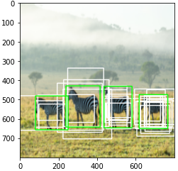
9) Non maximum suppression(select 2000 bounding boxes)
score 값이 높은걸 기준으로 IoU를 계산해주고 일정 이상값 이상이면 제외해줍니다.
# take all the roi boxes
x1 = roi[:, 0]
y1 = roi[:, 1]
x2 = roi[:, 2]
y2 = roi[:, 3]

# find the areas of all the boxes
areas = (x2 - x1 + 1) * (y2 - y1 + 1)


# take the indexes of order the probability score in descending order
# non maximum suppression
# 첫번째를 기준으로 iou값을 이용해 0.7 이하 값들로 다시 계산해준다.
order = order.argsort()[::-1] # 위에서 정렬을 해줬는데 왜 order에 argsort를 해주지?
keep = []

while (order.size > 0):
  i = order[0] # take the 1st elt in roder and append to keep
  keep.append(i)

  xx1 = np.maximum(x1[i], x1[order[1:]])
  yy1 = np.maximum(y1[i], y1[order[1:]])
  xx2 = np.minimum(x2[i], x2[order[1:]])
  yy2 = np.minimum(y2[i], y2[order[1:]])

  w = np.maximum(0.0, xx2 - xx1 + 1)
  h = np.maximum(0.0, yy2 - yy1 + 1)

  inter = w * h
  ovr = inter / (areas[i] + areas[order[1:]] - inter)
  inds = np.where(ovr <= nms_thresh)[0]
  order = order[inds + 1]

keep = keep[:n_train_post_nms] # while training/testing, use accordingly
roi = roi[keep]
Proposal Target Layer
10) FastR-CNN 모델을 학습시키기 위한 유용한 sample을 선택하는 것입니다. 학습을 위해 128개의 sample을 mini-batch로 구성합니다. 이 때 Proposal layer에서 얻은 anchor box 중 ground truth box와의 IoU 값이 0.5 이상인 box를 positive sample로, 0.5 미만인 box를 negative sample로 지정합니다(IoU를 구하는 과정은코드를 참고하시기 바랍니다). 전체 mini-batch sample 중 1/4, 즉 32개가 positive sample이 되도록 구성합니다.
# select the foreground rois as pre the pos_iou_thresh
# and n_sample x pos_ratio (128 x 0.25 = 32) foreground samples

pos_roi_per_image = 32
pos_index = np.where(max_iou >= pos_iou_thresh)[0]
pos_roi_per_this_image = int(min(pos_roi_per_image, pos_index.size))

if pos_index.size > 0:
  pos_index = np.random.choice(
      pos_index, size=pos_roi_per_this_image, replace=False)


# Select background negative samples
# similarly we do for negative(background) region proposals

neg_index = np.where((max_iou < neg_iou_thresh_hi) &
                     (max_iou >= neg_iou_thresh_lo))[0]
neg_roi_per_this_image = n_sample - pos_roi_per_this_image
neg_roi_per_this_image = int(min(neg_roi_per_this_image, neg_index.size))

if neg_index.size > 0:
  neg_index = np.random.choice(
    neg_index, size = neg_roi_per_this_image, replace=False)
RoI pooling
11) Feature extractor를 통해 얻은 feature map과 Proposal Target layer에서 추출한 region proposals을 활용하여 RoI pooling을 수행합니다. 이 때 output feature map의 크기가 7x7이 되도록 설정합니다.
size = (7, 7)
adaptive_max_pool = nn.AdaptiveMaxPool2d(size[0], size[1])

output = []
rois = indices_and_rois.data.float()
rois[:, 1:].mul_(1/16.0) # sub-sampling ratio
rois = rois.long()
num_rois = rois.size(0)

for i in range(num_rois):
  roi = rois[i]
  im_idx = roi[0]
  im = output_feature.narrow(0, im_idx, 1)[..., roi[1]:(roi[3]+1), roi[2]:(roi[4]+1)]
  tmp = adaptive_max_pool(im)
  output.append(tmp[0])

output = torch.cat(output, 0)


