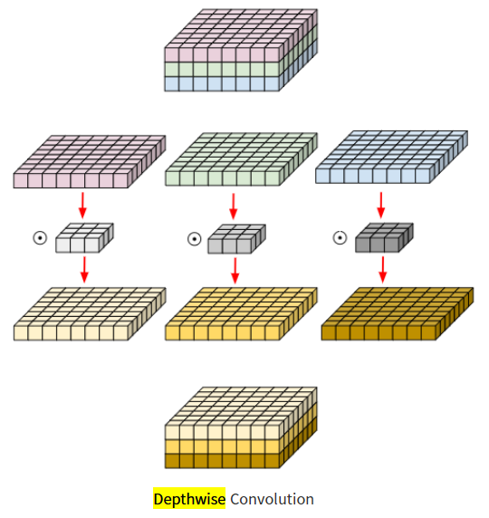
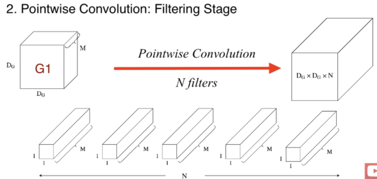
1. Depthwise Separable Convolution
def depthwise_separable_conv(input_dim, output_dim):

    depthwise_convolution = nn.Conv2d(input_dim, input_dim, kernel_size=3, padding=1, groups=input_dim, bias=False)
    pointwise_convolution = nn.Conv2d(input_dim, output_dim, kernel_size=1, bias=False)

    model = nn.Sequential(
        depthwise_convolution,
        pointwise_convolution

    )

    return model
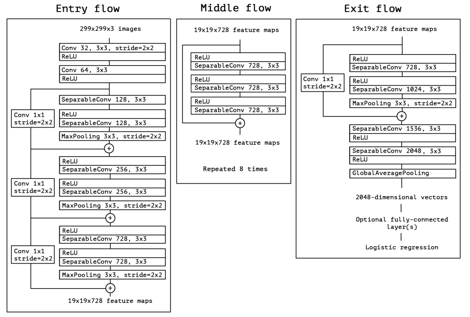
2. Entry flow
class entry_flow(nn.Module):
    def __init__(self):
        super(entry_flow, self).__init__()

        self.conv2d_init_1 = nn.Conv2d(in_channels = 3,
                                       out_channels = 32,
                                       kernel_size = 3,
                                       stride = 2,
                                      )

        self.conv2d_init_2 = nn.Conv2d(in_channels = 32,
                                       out_channels = 64,
                                       kernel_size = 3,
                                       stride = 1,
                                      )


        self.layer_1 = nn.Sequential(
            depthwise_separable_conv(input_dim = 64, output_dim = 128),
            nn.ReLU(),
            depthwise_separable_conv(input_dim = 128, output_dim = 128),
            nn.MaxPool2d(kernel_size=3, stride=2, padding=1)

        )

        self.conv2d_1 = nn.Conv2d(in_channels = 64,
                                  out_channels = 128,
                                  kernel_size = 1,
                                  stride = 2
                                  )

        self.layer_2 = nn.Sequential(
            depthwise_separable_conv(input_dim = 128, output_dim = 256),
            nn.ReLU(),
            depthwise_separable_conv(input_dim = 256, output_dim = 256),
            nn.MaxPool2d(kernel_size=3, stride=2, padding=1)

        )

        self.conv2d_2 = nn.Conv2d(in_channels = 128,
                                  out_channels = 256,
                                  kernel_size = 1,
                                  stride = 2
                                  )

        self.layer_3 = nn.Sequential(
            depthwise_separable_conv(input_dim = 256, output_dim = 728),
            nn.ReLU(),
            depthwise_separable_conv(input_dim = 728, output_dim = 728),
            nn.MaxPool2d(kernel_size=3, stride=2, padding=1)

        )

        self.conv2d_3 = nn.Conv2d(in_channels = 256,
                                  out_channels = 728,
                                  kernel_size = 1,
                                  stride = 2
                                  )

        self.relu = nn.ReLU()

    def forward(self, x):
        x = self.conv2d_init_1(x)
        x = self.relu(x)
        x = self.conv2d_init_2(x)
        x = self.relu(x)

        output1_1 = self.layer_1(x)
        output1_2 = self.conv2d_1(x)
        output1_3 = output1_1 + output1_2


        output2_1 = self.layer_2(output1_3)
        output2_2 = self.conv2d_2(output1_3)
        output2_3 = output2_1 + output2_2


        output3_1 = self.layer_3(output2_3)
        output3_2 = self.conv2d_3(output2_3)
        output3_3 = output3_1 + output3_2
        y = output3_3

        return y
3. Middle flow
class middle_flow(nn.Module):
    def __init__(self):
        super(middle_flow, self).__init__()

        self.module_list = nn.ModuleList()

        layers = nn.Sequential(
                nn.ReLU(),
                depthwise_separable_conv(input_dim = 728, output_dim = 728),
                nn.ReLU(),
                depthwise_separable_conv(input_dim = 728, output_dim = 728),
                nn.ReLU(),
                depthwise_separable_conv(input_dim = 728, output_dim = 728)
            )

        for i in range(7):
            self.module_list.append(layers)

    def forward(self, x):
        for layer in self.module_list:
            x_temp = layer(x)
            x = x + x_temp

        return x
4. Exit flow
class exit_flow(nn.Module):
    def __init__(self, growth_rate=32):
        super(exit_flow, self).__init__()

        self.separable_network = nn.Sequential(
            nn.ReLU(),
            depthwise_separable_conv(input_dim = 728, output_dim = 728),
            nn.ReLU(),
            depthwise_separable_conv(input_dim = 728, output_dim = 1024),
            nn.MaxPool2d(kernel_size=3, stride=2, padding=1)
        )

        self.conv2d_1 = nn.Conv2d(in_channels = 728,
                                  out_channels = 1024,
                                  kernel_size = 1,
                                  stride = 2
                                  )

        self.separable_conv_1 = depthwise_separable_conv(input_dim = 1024, output_dim = 1536)
        self.separable_conv_2 = depthwise_separable_conv(input_dim = 1536, output_dim = 2048)

        self.relu = nn.ReLU()
        self.avgpooling = nn.AdaptiveAvgPool2d((1))

        self.fc_layer = nn.Linear(2048, 10)

    def forward(self, x):
        output1_1 = self.separable_network(x)
        output1_2 = self.conv2d_1(x)
        output1_3 = output1_1 + output1_2

        y = self.separable_conv_1(output1_3)
        y = self.relu(y)
        y = self.separable_conv_2(y)
        y = self.relu(y)
        y = self.avgpooling(y)

        y = y.view(-1, 2048)
        y= self.fc_layer(y)


        return y
5. Xception
class Xception(nn.Module):
    def __init__(self):
        super(Xception, self).__init__()
        self.entry_flow = entry_flow()
        self.middle_flow = middle_flow()
        self.exit_flow = exit_flow()


    def forward(self, x):
        x = self.entry_flow(x)
        x = self.middle_flow(x)
        x = self.exit_flow(x)

        return x